COILED COIL tutorial
Aims of the tutorial
This tutorial shows how to launch the coiled_coil mode1 implemented in ARCIMBOLDO_LITE2 in order to solve ab initio a 128 aminoacids structure at 2.5Å and analyse the output of the program. This example uses the ARCIMBOLDO_LITE version released on November 2018 through CCP4/our website.
Data tutorial
Experimental details
Test data for our tutorial is the crystal structure of the vDED coiled coil domain from human BAP29. BAP29 is a protein that resides in the endoplasmic reticulum and is involved in regulating intracellular sorting of several membrane proteins. The structure is composed by 2 α-helices wrapped around each other to form a coiled coil domain, and is deposited in the Protein Data Bank under the PDB code 4W7T3.
Details of the data are summarized in the following table:
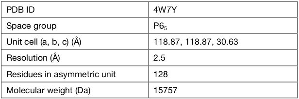
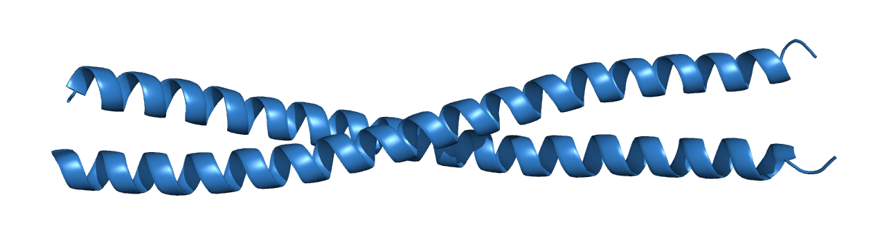
Figure 1. Cartoon representation of PDB entry 4W7Y. This figure was prepared using Pymol4.
Step by Step tutorial
For this tutorial we will need only the reflection file in two formats (.mtz and .hkl). All required files can be downloaded here. The model to search will be ideal helices that are defined internally in the program just from its length. After downloading ARCIMBOLDO_LITE (see instructions here), you are ready to follow this tutorial.
Input
We need 3 files in order to run ARCIMBOLDO_LITE:
Configuration .bor file:
The configuration file looks like follows:
[CONNECTION]:
distribute_computing: multiprocessing
setup_file: /path/to/setup.bor

[GENERAL]:
working_directory: /path/to/working_directory
mtz_path: %(working_directory)s/data.mtz
hkl_path: %(working_directory)s/data.hkl

[ARCIMBOLDO]
name_job: 4w7y
molecular_weight: 15757
number_of_component: 1
f_label: FOBS
sigf_label: SIGFOBS
fragment_to_search: 2
helix_length: 18
shelxe_line = -m10 -a8 -s0.6 -v0 -t10 -Q -I10 -y2.50 -e2.20 -f
coiled_coil: true

[LOCAL]
path_local_phaser: /path/to/phaser
path_local_shelxe: /path/to/shelxe
The [CONNECTION] section specifies the computing system used and the file containing the general configuration. The job can be run on a single machine (in multiprocessing) or in a local or remote grid of computers.If you want to run the job in multiprocessing you just have to change in the .bor file that you downloaded the paths of the working directory, phaser and shelxe.
The [GENERAL] section contains the .mtz and .hkl file paths as well as the working directory where results will be written.
In the [ARCIMBOLDO] section all parameterization for the job is specified:
- RMSD set to 0.2Å (rmsd: 0.2)
- VRMS calculation in the refinement step to optimize the RMSD parameter in order to maximize the LLG.
- Disable placing pairs of tNCS related helices, as the internal periodicity of a single helix makes difficult to differentiate genuine intermolecular tNCS from Patterson artefacts. If no solution is achieved, the alternative should be tried.
- Activation of PHASER’s packing filter at translation, so at least one translated solution will pass the packing check.
- Generate and probe reverse helices. At resolution below 2 Å it was frequently observed that placement of the first helices occasionally took place in the correct position but in reversed direction and at low resolution are not distinguishable from the PHASER figures of merit.
- Final verification step, an additional step that generates perturbations of the substructure leading to the best solution andcompares their scores before and after extension. As the reverse helices this will be only activated at resolution worse than 2Å.
- SHELXE with helical sliding, which improves the autotracing of the coiled coil structures.
Finally, in the [LOCAL] section, the paths to PHASER and SHELXE are set. This is only required if you are in multiprocessing mode.
Execution
You can run the program interactively, having the output displayed on the screen or do it in background, redirecting an input file and passing the output to a .log file.
1. Interactively:
ARCIMBOLDO_LITE 4w7y.bor
2. In background:
nohup ARCIMBOLDO_LITE 4w7y.bor >& logfile.log;
Output and Results
ARCIMBOLDO_LITE will generate several files related to the PHASER and SHELXE runs. For each step in the search (rotation, translation, packing, etc), there will be a folder with the output.
The html output file summarizes your job instructions and results. This file is updated during the run and can be opened in an internet browser.
A brief summary of the data follows, showing the input space group, cell dimensions, resolution and number of reflections.
After this summary, there is a table for each fragment in which the rotation clusters found are listed along with their figures of merit at each step of the process. The tables are updated in real time and can serve to judge parameterization.
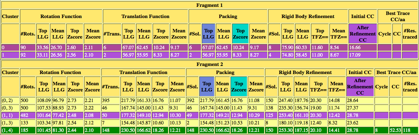
Figure 2. Interactive table with the figures of merit from PHASER6 and SHELXE7 for each rotation cluster.
After the table you can observe the backtrace and figures of merit for the best solution, in this case the structure is solved with a CC of 51.78% and 127 residues traced. Also there are links to access the best scoring solution: the .pdb of the traced structure and its map in .phs format.
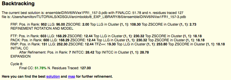
Figure 3. Backtracing of the model that leads to a correct solution.
Following the backtracing, there is a verification graph saying that the verification step has determined that the structure is solved because in this case the best solution is clearly distinguished from a random one.
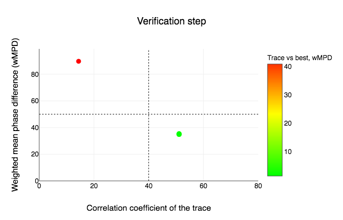
Figure 4. Verification step graph.
Finally, the last section of the html contains a full configuration file will be reported showing the parametrization that the user configured as well as the defaults that remained unchanged, and the log file of the run.
References
-
ARCIMBOLDO on coiled coils.
Caballero, I., Sammito, M., Millan, C., Lebedev, A., Soler, N. and Uson, I.
Acta Cryst. D74, 194-204 (2018) (doi:10.1107/S2059798317017582)
-
ARCIMBOLDO_LITE: single-workstation implementation and use.
Sammito, M., Millán, C., Frieske, D., Rodríguez-Freire, E., Borges, R. J. and Usón, I.
Acta Cryst. D71, 1921-30 (2015) (doi: 10.1107/S1399004715010846)
-
A disulfide polymerized protein crystal.
Quistgaard, EM.
Chem Commun (Camb), 14995-7 (2014) (doi: 10.1039/c4cc07326f)
-
The PyMOL Molecular Graphics System.
Version 1.5.0.4 Schrödinger, LLC. (https://pymol.org)
-
Overview of the CCP4 suite and current developments.
Winn, M.D. et al.
Acta Cryst. D67, 235-242 (2011) (doi: 10.1107/S0907444910045749)
-
Phaser crystallographic software.
McCoy, A. J., Grosse-Kunstleve, R. W., Adams, P. D., Winn, M. D., Storoni, L. C. and Read, R. J.
J. Appl. Crystallogr. D40, 658-674 (2007) (doi: 10.1107/S0021889807021206)
-
An introduction to experimental phasing of macromolecules illustrated by SHELX; new autotracing features.
Uson, I. and Sheldrick, G.M.
Acta Cryst. D74, 106-116 (2018) (doi: 10.1107/S2059798317015121)