ALIXE tutorial
Aims of the tutorial
This tutorial shows how to use ALIXE as a standalone program to combine partial solutions coming from an ARCIMBOLDO_SHREDDER spherical run. ALIXE orders all putative solutions by their figures of merit, compares all of them and combines those within a given similarity threshold to the cluster formed. The process is iterative and solutions may enter or exit a cluster, as the phases of the combined cluster change. This example uses the latest ALIXE as of March 2020 and the solutions obtained with the ARCIMBOLDO_SHREDDER spherical tutorial from this website.
Step by Step tutorial
1. Perform the ARCIMBOLDO_SHREDDER spherical tutorial solving the Slt lytic transglycosylase from Pseudomonas aeruginosa (PDB id 5OHU) http://chango.ibmb.csic.es/tutorial_shredder_spherical
2. Use ALIXE
Required input (minimal command line or a configuration file)
- To run in the command line:
If 5ohu_spheres.bor does not have a [LOCAL] section, ALIXE will assume that the path to the SHELXE executable has been defined (e.g. within CCP4).ALIXE -m monomer -i path/to/5ohu_spheres.bor
- The configuration .bor file:
[ALIXE]
[input_info_1]: path/to/5ohu_spheres.bor
[alixe_mode]: monomer
The configuration .bor file is generated running:
ALIXE.py -f name_conf.bor
It contains all parameters and their pertinent keywords described in the manual.
This tutorial runs ALIXE using a minimal input. The minimal configuration bor file requires:
- the path to the configuration bor file of the ARCIMBOLDO_SHREDDER run
- the ALIXE mode
In addition, any keyword from the manual can be added to the configuration bor file.
Rotation clustering in ARCIMBOLDO allows separating putative partial solutions that would correspond to a single copy of the molecule in the asymmetric unit from those that would map to different copies in a multimer. Therefore, in a monomer mode, the phase comparison is limited to partial solutions within the same rotation cluster, while the multimer mode compares the resulting output of a previous monomer clustering.
This particular case entails the use of the monomer mode, as crystals contain one single copy of 5OHU in the asymmetric unit.
Execution
With an ALIXE bor file:
- Interactively:
- In the background:
ALIXE.py 5ohu_alixe.bor
ALIXE.py 5ohu_alixe.bor >& log &
By minimal command line:
ALIXE.py -m monomer -i 5ohu.bor
Output and Results
By default, a folder called CLUSTERING will be written in the working directory where you launch ALIXE. Consider that a preexisting folder called CLUSTERING will be overwritten unless a new name for the output folder is given explicitly.
This output folder contains the log file autoalixe.log, which shows that the job has finished (and quotes the time taken). It will display the CC characterising the best solution and if this figure is higher than 30% (and therefore the structure is presumably solved) relevant information about this cluster and the output files to retrieve are provided.
The command line used to generate the run is also echoed.
* Info *  Output folder will be /Path/to/CLUSTERING

* Info *  Achieved a CC of 32.09%

* Info *  The structure was possibly solved, check frag590_0_0_rbr_0_ref.lst

* Info *
Total time spent in running autoalixe is 152 minutes
Command line used was /Path/to/ARCIMBOLDO_FULL/ALIXE.py alixe_tutorial.bor
Along with the log output, a directory called clustpool_1 gathers all partial solutions with the extension pda, their associated phase sets with the extension .phs and the phase clusters produced ending as .phi. In addition, there are two tables that supply information either about the single solutions and combinations.
| Name | LLGrbr | LLGgimb | Z-score | Rotcluster | InitCC | Efom | PseudoCC |
|---|---|---|---|---|---|---|---|
| frag590_0_0_rbr_0 | 92.5 | 143.8 | 7.21 | 0 | 9.9 | 0.202 | 23.43 |
| frag595_0_0_rbr_0 | 87.0 | 106.2 | 7.93 | 0 | 8.91 | 0.226 | 25.75 |
| frag591nogyre_0_0_rbr_01 | 84.4 | 84.5 | 8.68 | 0 | 7.89 | 0.202 | 23.95 |
| ... | ... | ... | ... | ... | ... | ... | ... |
Table 1. Table clustpool_1_info_frag.
It summarizes the figures of merit of the partial solutions that are being combined.
| Cluster | n_phs | topzscore | topllg |
|---|---|---|---|
| frag590_0_0_rbr_0_ref.phi | 66 | 9.07 | 143.8 |
| frag213nogyre_0_0_rbr_2_ref.phi | 5 | 4.73 | 28.7 |
| frag226nogyre_0_0_rbr_2_ref.phi | 4 | 4.71 | 22.6 |
| frag331nogyre_0_0_rbr_0_ref.phi | 4 | 4.91 | 25.1 |
| frag44nogyre_0_0_rbr_3_ref.phi | 4 | 4.19 | 25.1 |
| frag174nogyre_0_0_rbr_0_ref.phi | 3 | 4.42 | 29.4 |
| frag258nogyre_0_0_rbr_3_ref.phi | 3 | 4.94 | 28.3 |
| frag285nogyre_0_0_rbr_2_ref.phi | 3 | 5.26 | 25.8 |
| frag297nogyre_0_0_rbr_2_ref.phi | 3 | 5.2 | 27.6 |
| frag326nogyre_0_0_rbr_1_ref.phi | 3 | 5.02 | 27.9 |
| frag383nogyre_0_0_rbr_2_ref.phi | 3 | 4.65 | 26.9 |
| frag399nogyre_0_0_rbr_2_ref.phi | 3 | 4.97 | 31.7 |
| frag424nogyre_0_0_rbr_0_ref.phi | 3 | 4.11 | 22.7 |
| frag46nogyre_0_0_rbr_3_ref.phi | 3 | 4.21 | 23.9 |
| frag103nogyre_0_0_rbr_2_ref.phi | 2 | 4.66 | 25.2 |
| frag122nogyre_0_0_rbr_3_ref.phi | 2 | 4.15 | 22.9 |
| frag146nogyre_0_0_rbr_1_ref.phi | 2 | 4.39 | 21.2 |
| frag161nogyre_0_0_rbr_0_ref.phi | 2 | 4.87 | 26.4 |
| frag191nogyre_0_0_rbr_2_ref.phi | 2 | 4.37 | 23.7 |
| frag191nogyre_0_0_rbr_3_ref.phi | 2 | 4.29 | 26.1 |
| frag202nogyre_0_0_rbr_2_ref.phi | 2 | 4.29 | 23.5 |
| frag205nogyre_0_0_rbr_0_ref.phi | 2 | 4.52 | 23.6 |
| frag220nogyre_0_0_rbr_0_ref.phi | 2 | 4.73 | 25.8 |
| frag235nogyre_0_0_rbr_3_ref.phi | 2 | 4.65 | 22.7 |
| frag251nogyre_0_0_rbr_3_ref.phi | 2 | 4.07 | 21.7 |
| frag261nogyre_0_0_rbr_3_ref.phi | 2 | 4.59 | 22.3 |
| frag276nogyre_0_0_rbr_0_ref.phi | 2 | 4.75 | 25.5 |
| frag27nogyre_0_0_rbr_2_ref.phi | 2 | 4.7 | 27.2 |
| frag293nogyre_0_0_rbr_0_ref.phi | 2 | 5.06 | 24 |
| frag293nogyre_0_0_rbr_3_ref.phi | 2 | 4.67 | 21.4 |
| frag29nogyre_0_0_rbr_2_ref.phi | 2 | 4.34 | 25.8 |
| frag305nogyre_0_0_rbr_2_ref.phi | 2 | 4.37 | 18.5 |
| frag344nogyre_0_0_rbr_1_ref.phi | 2 | 4.57 | 23.5 |
| frag351nogyre_0_0_rbr_1_ref.phi | 2 | 5.37 | 33.3 |
| frag420nogyre_0_0_rbr_0_ref.phi | 2 | 4.61 | 25 |
| frag421nogyre_0_0_rbr_0_ref.phi | 2 | 4.41 | 19.1 |
| frag421nogyre_0_0_rbr_3_ref.phi | 2 | 4.49 | 22.9 |
| frag425nogyre_0_0_rbr_2_ref.phi | 2 | 4.76 | 24.9 |
| frag475nogyre_0_0_rbr_3_ref.phi | 2 | 4.14 | 20.1 |
| frag563nogyre_0_0_rbr_2_ref.phi | 2 | 5.19 | 29.1 |
| frag573nogyre_0_0_rbr_1_ref.phi | 2 | 4.6 | 26.4 |
| frag577nogyre_0_0_rbr_0_ref.phi | 2 | 4.23 | 21.6 |
| frag596nogyre_0_0_rbr_1_ref.phi | 2 | 4.63 | 21.9 |
| frag6nogyre_0_0_rbr_0_ref.phi | 2 | 4.37 | 23.3 |
| frag70nogyre_0_0_rbr_2_ref.phi | 2 | 4.9 | 29.9 |
| frag7nogyre_0_0_rbr_2_ref.phi | 2 | 4.41 | 24.5 |
| frag8nogyre_0_0_rbr_0_ref.phi | 2 | 4.24 | 21.2 |
Table 2. Table clustpool_1_info_clust_table.
This table shows information about the scores of the clusters and number of phase sets combined in each cluster. Here we omit the single solutions.The cluster is named after the phase set used as a reference to initiate it, n_phs refers to the number of phase sets that have been joined in each cluster and topzscore and topllg are the top Z-score and LLG values found in the group of solutions.
Notice that there is a cluster gathering a majority of phase sets. This is a promising indication as phases from a correct partial structure should approximate the true structure and, therefore, should be more consistent than to those relating misplaced models.
Whenever the figures of merit scoring the partial solutions are available, as in the present case, ALIXE will produce graphical output of the landscape of solutions in png format. Three plots will be displayed, two for single solutions and one for the clusters produced.
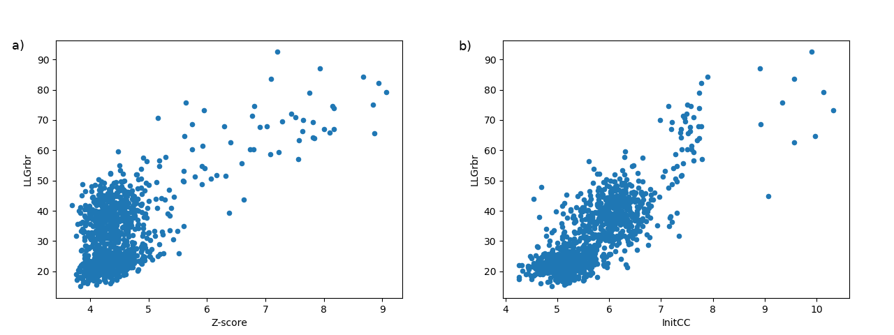
Figure 1.
Examples illustrating typical landscapes of partial solutions rendered by phasing with fragments. The points in the scatter plots represent single partial solutions from an ARCIMBOLDO-SHREDDER run. The ordinate shows the LLG score after rigid-body refinement and the abscissa shows the Z-score (a) and the correlation coefficient (b). (a)(b) Plots representing the distribution of single partial solutions.

Figure 2.
Scatter plot representing the clusters produced by ALIXE from the putative solutions represented in Figure 1. The ordinate shows the LLG score after rigid-body refinement and the abscissa shows the Z-score. In this particular plot, the single, large cluster produced, showing top figures of merit conforms an ideal positive outcome.
These plots (Figure 1) enable an intuitive understanding of the global scenario of the partial solutions. A promising scenario will show some distinction among the probes, revealing single partial solutions crearly detached from the rest and presenting higher figures of merit.
They produce a better insight when combined with the plot (Figure 2) with the information from the clusters. Clusters gathering a large number of solutions and including the best scored ones are a positive indication (large circles close to the top right corner). The plot representing the phase clusters also shows clearly the reduction of partial solutions achieved, leading to a time reduction spent to process them.
The keyword expansions is set to True by default meaning clusters will be trialled through density modification and autotracing, possibly revealing a full correct and complete solution. Nevertheless, as in fragment-based molecular replacement probes are not independent large clusters may still correspond to incorrect probes that are consistently related.
In this tutorial, one particularly large cluster has been produced, along with many smaller clusters with poorer scores. The large cluster produced is very likely a non-random solution. Nevertheless, it is not possible to assert correctness until performing density modification and autotracing with SHELXE. If the unknown structure is solved after density modification and autotracing with SHELXE the following message will be displayed in the autoalixe.log file:
* Info *  Achieved a CC of 32.09%

* Info *  The structure was possibly solved, check frag590_0_0_rbr_0_ref.lst

* Info *
Total time spent in running autoalixe is 152 minutes
 Command line used was /Path/to/ARCIMBOLDO_FULL/ALIXE.py alixe_tutorial.bor
Achieving a correlation coefficient (CC) higher than 30% reveals that the structure is solved for the data resolution in this example.
Also there is a directory called clustpool_n (where n is an integer). In this case clustpool_1 as only one input_info is given. Inside this directory you will find your partial solutions in real space with the extension pda, their phase sets associated with the phs extension and the clusters generated from its combination ending as .phi. If the parameter fusecoord is set to True you will also find files ending with shifted.pda that will correspond to an equivalent of each cluster produced in real space.
In addition, there are two tables that supply information either about the single solutions and the clusters produced.
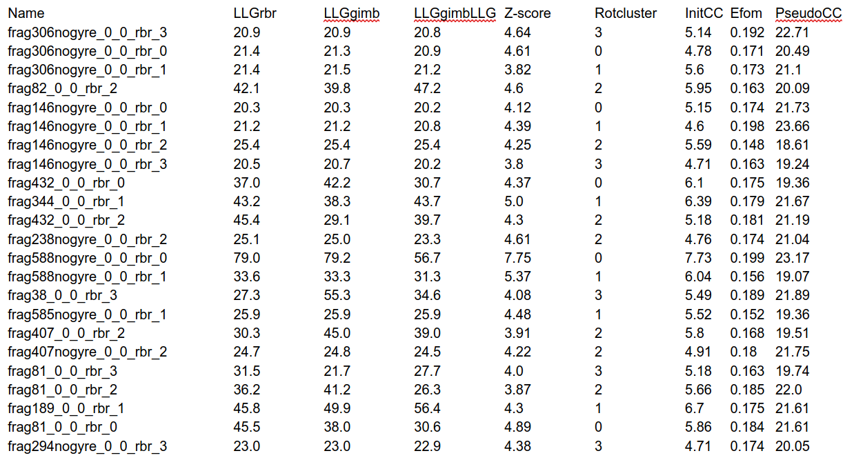
Table 3. clustpool_1_info_frag
It provides information about the figures of merit of the partial solutions that are being combined.
| Cluster | n_phs | topzscore | topllg | fused_cc | phi_cc |
|---|---|---|---|---|---|
| frag103nogyre_0_0_rbr_2_ref.phi | 2 | 4.66 | 25.2 | 2.58 | -1 |
| frag122nogyre_0_0_rbr_3_ref.phi | 2 | 4.15 | 22.8 | 2.42 | -1 |
| frag146nogyre_0_0_rbr_1_ref.phi | 2 | 4.39 | 20.8 | 1.74 | -1 |
| frag161nogyre_0_0_rbr_0_ref.phi | 2 | 4.87 | 25.7 | 2.79 | -1 |
| frag191nogyre_0_0_rbr_2_ref.phi | 2 | 4.37 | 23.5 | 2.27 | -1 |
| frag191nogyre_0_0_rbr_3_ref.phi | 2 | 4.29 | 25.8 | 2.8 | -1 |
| frag202nogyre_0_0_rbr_2_ref.phi | 2 | 4.29 | 23.4 | 2.02 | -1 |
| frag205nogyre_0_0_rbr_0_ref.phi | 2 | 4.52 | 23.5 | 2.3 | -1 |
| frag220nogyre_0_0_rbr_0_ref.phi | 2 | 4.73 | 25.6 | 2.52 | -1 |
| frag235nogyre_0_0_rbr_3_ref.phi | 2 | 4.65 | 22.7 | 2.14 | -1 |
| frag251nogyre_0_0_rbr_3_ref.phi | 2 | 4.07 | 21.7 | 2.45 | -1 |
| frag261nogyre_0_0_rbr_3_ref.phi | 2 | 4.59 | 22 | 2.32 | -1 |
| frag276nogyre_0_0_rbr_0_ref.phi | 2 | 4.75 | 24.9 | 2.5 | -1 |
| frag27nogyre_0_0_rbr_2_ref.phi | 2 | 4.7 | 27.2 | 2.79 | -1 |
| frag293nogyre_0_0_rbr_0_ref.phi | 2 | 5.06 | 23.7 | 2.65 | -1 |
| frag293nogyre_0_0_rbr_3_ref.phi | 2 | 4.67 | 21 | 1.78 | -1 |
| frag29nogyre_0_0_rbr_2_ref.phi | 2 | 4.34 | 25.8 | 2.71 | -1 |
| frag305nogyre_0_0_rbr_2_ref.phi | 2 | 4.37 | 18.4 | 2.61 | -1 |
| frag344nogyre_0_0_rbr_1_ref.phi | 2 | 4.57 | 23.5 | 1.94 | -1 |
| frag351nogyre_0_0_rbr_1_ref.phi | 2 | 5.37 | 31.3 | 3.13 | -1 |
| frag420nogyre_0_0_rbr_0_ref.phi | 2 | 4.61 | 24.6 | 2.34 | -1 |
| frag421nogyre_0_0_rbr_0_ref.phi | 2 | 4.41 | 18.9 | 2.96 | -1 |
| frag421nogyre_0_0_rbr_3_ref.phi | 2 | 4.49 | 22.7 | 2.26 | -1 |
| frag425nogyre_0_0_rbr_2_ref.phi | 2 | 4.76 | 24.9 | 2.81 | -1 |
| frag475nogyre_0_0_rbr_3_ref.phi | 2 | 4.14 | 20 | 1.86 | -1 |
| frag563nogyre_0_0_rbr_2_ref.phi | 2 | 5.19 | 27.9 | 3.12 | -1 |
| frag573nogyre_0_0_rbr_1_ref.phi | 2 | 4.6 | 26.2 | 2.85 | -1 |
| frag577nogyre_0_0_rbr_0_ref.phi | 2 | 4.23 | 21.4 | 2.44 | -1 |
| frag596nogyre_0_0_rbr_1_ref.phi | 2 | 4.63 | 21.3 | 2.92 | -1 |
| frag6nogyre_0_0_rbr_0_ref.phi | 2 | 4.37 | 23.3 | 2.34 | -1 |
| frag70nogyre_0_0_rbr_2_ref.phi | 2 | 4.9 | 29.9 | 2.83 | -1 |
| frag7nogyre_0_0_rbr_2_ref.phi | 2 | 4.41 | 24.5 | 2.51 | -1 |
| frag8nogyre_0_0_rbr_0_ref.phi | 2 | 4.24 | 21.2 | 1.93 | -1 |
| frag174nogyre_0_0_rbr_0_ref.phi | 3 | 4.42 | 28.8 | 2.42 | -1 |
| frag258nogyre_0_0_rbr_3_ref.phi | 3 | 4.94 | 27.8 | 2.99 | -1 |
| frag285nogyre_0_0_rbr_2_ref.phi | 3 | 5.26 | 25.7 | 2.24 | -1 |
| frag297nogyre_0_0_rbr_2_ref.phi | 3 | 5.2 | 27 | 3.42 | -1 |
| frag326nogyre_0_0_rbr_1_ref.phi | 3 | 5.02 | 27.4 | 2.51 | -1 |
| frag383nogyre_0_0_rbr_2_ref.phi | 3 | 4.65 | 26.9 | 2.9 | -1 |
| frag399nogyre_0_0_rbr_2_ref.phi | 3 | 4.97 | 30.7 | 3.74 | -1 |
| frag424nogyre_0_0_rbr_0_ref.phi | 3 | 4.11 | 22.4 | 2.19 | -1 |
| frag46nogyre_0_0_rbr_3_ref.phi | 3 | 4.21 | 23.6 | 2.06 | -1 |
| frag226nogyre_0_0_rbr_2_ref.phi | 4 | 4.71 | 22.7 | 2.63 | -1 |
| frag331nogyre_0_0_rbr_0_ref.phi | 4 | 4.91 | 25.1 | 1.77 | -1 |
| frag44nogyre_0_0_rbr_3_ref.phi | 4 | 4.19 | 25.1 | 2.41 | -1 |
| frag213nogyre_0_0_rbr_2_ref.phi | 5 | 4.73 | 28.7 | 2.08 | -1 |
| frag590_0_0_rbr_0_ref.phi | 66 | 9.07 | 87.5 | 7.33 | -1 |
Table 4. clustpool_1_info_clust_table
The clustpool_1_info_clust_table shows information about the scores of the clusters produced. Here we only show the clusters that joined at least 2 solutions and omit the single solutions. In this table, the column named cluster corresponds to the cluster, named after the phase set that has been used as a reference to form it, n_phs refers to the number of phase sets that have been joined in each cluster and topzscore and topllg are the largest Z-score and LLG found in that group of solutions.
If the keyword plots is set to True and figures of merit of partial solutions are available, ALIXE will produce graphical output of the landscape of your solutions taking into account their scores. Four graphics will be displayed in pdf format, two for single solutions and two for the clusters produced.
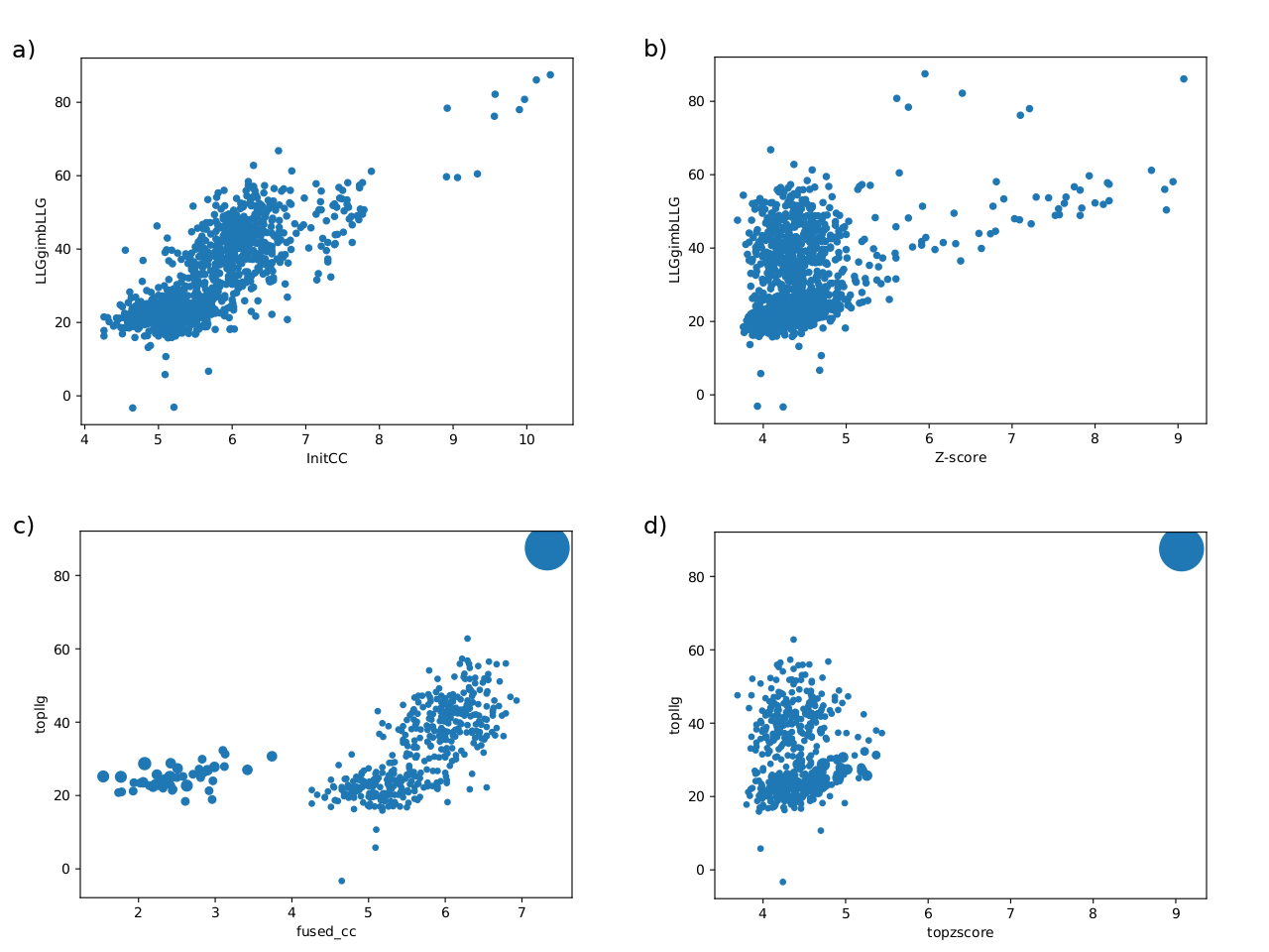
Figure 3.
Examples illustrating typical landscapes of partial solutions rendered by phasing with fragments. The points in the scatter plots represent either single partial solutions (a)(b) orclusters of partial solutions (c)(d) from an ARCIMBOLDO-SHREDDER run. The ordinate shows the LLG score after rigid-body refinement and the abscissa shows the correlation coefficient (a)(c) and the Z-score (b)(d).
(a)(b) Plots representing the distribution of single partial solutions.
(c)(d) Plots representing the distribution of clusters.
In these particular plots, the single, large cluster produced, showing top figures of merit conforms a typical positive outcome.
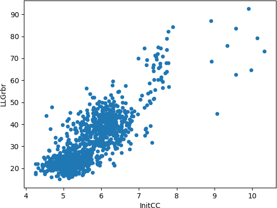
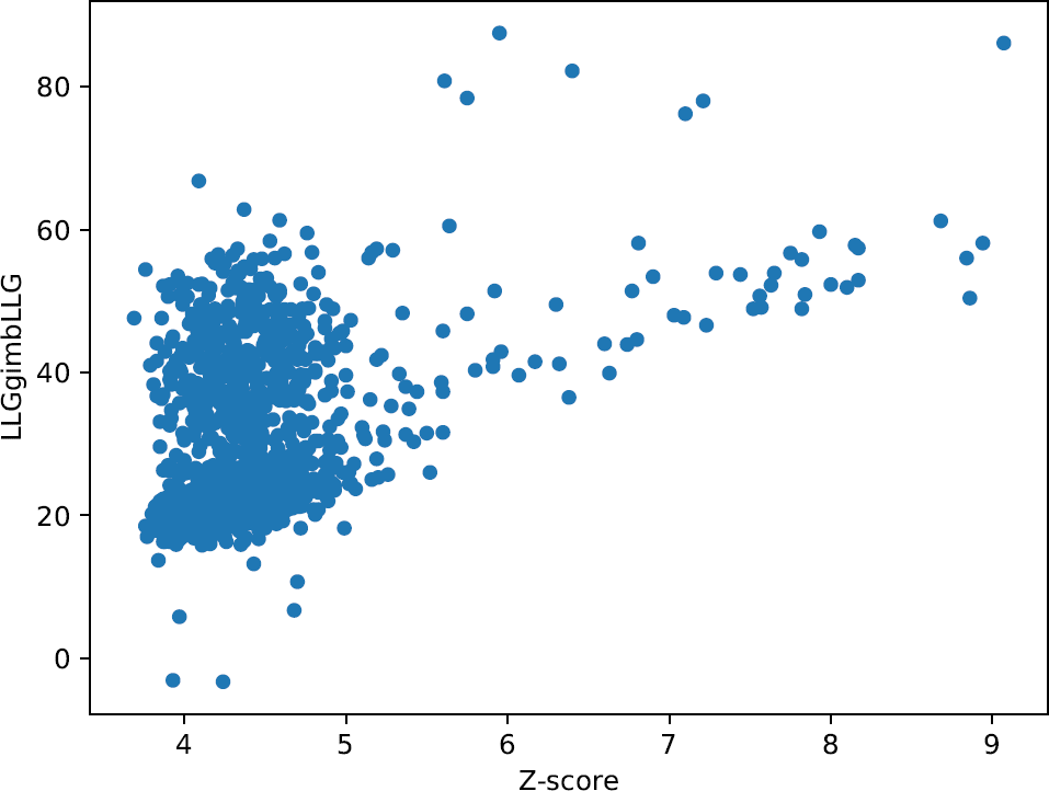
Figure 4.
These plots enable an intuitive understanding of the global scenario of the partial solutions, giving the opportunity to inquire if you have any possible correct solutions within the run. Any good-looking scenario will show some distinction between all probes, revealing single partial solutions crearly detached from the rest and presenting better figures of merit. They produce a better insight when combined with the plots drawn up with the information from the clusters. In this particular case, these graphics representing single solutions show probes with clearly better scores than the majority of them, reaching Z-scores higher than 7 and LLGs higher than 60. A landscape with this appearance could indicate a distinction between random and non random probes.
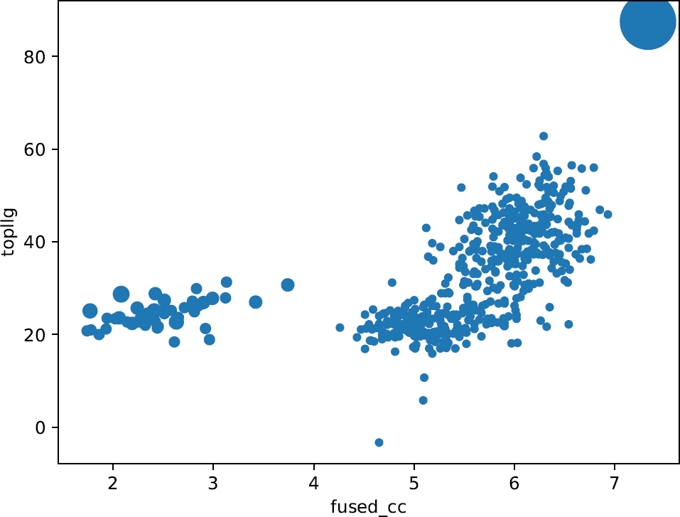
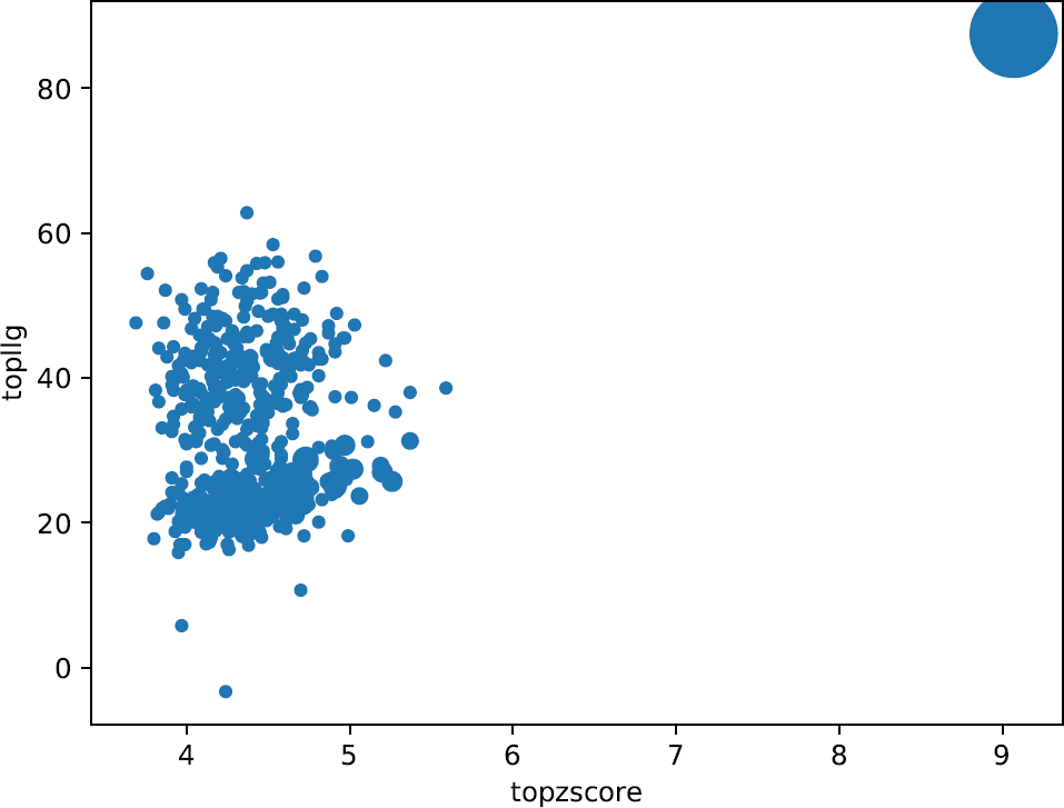
Figure 5.
These plots enable an intuitive understanding of the global scenario of the partial solutions, giving the opportunity to inquire if you have possibly correct solutions within the whole set. Any good-looking scenario will show some distinction between all probes, revealing single partial solutions crearly detached from the rest and presenting better figures of merit.
They produce a better insight when combined with the plots drawn up with the information from the clusters. The plots representing the phase clusters show clearly how the reduction of partial solutions is achieved, reducing also the time spent to process them. They represent with circles the clusters, and their radius is proportional to the number of phase sets that have been combined in each of them. Bigger circles (with a larger number of joined phase sets) might be indicative of possible success because true phase sets should be consistent with each other when referred to a common origin. Additionally, the clusters are plotted taking into account the top score reached by one the phase sets inside each cluster. Big clusters complemented with some discrimination between them is an apparent indication of a good scenario and if the keyword expansions is set to True, those clusters will be trialled for density modification and autotracing, possibly revealing a full correct and complete solution. Nevertheless, as in fragment-based molecular replacement probes are not independent big clusters may still correspond to incorrect probes that are consistently related.
Following the example we are using in this tutorial, it can be observed that one particularly large cluster has been produced together with a lot of smaller clusters with poorer scores. Such high scores in a large cluster might indicate very likely a non-random cluster. Nevertheless, it is not possible to assert correctness until performing density modification and autotracing with SHELXE. But the observation of large, discriminated clusters is an apparent indication of a good scenario that can be tested setting the expansions to True.
If the unknown structure is solved after density modification and autotracing with SHELXE the following message will be displayed on the terminal (if you have run ALIXE interactively) or at the end of the log file (if you have redirected ALIXE and run it in background):
frag590_0_0_rbr_0_ref.lst  has a CC after autotracing of  34.66

Achieved a CC of  34.66 %

The structure was possibly solved, check  frag590_0_0_rbr_0_ref.lst

Total time spent in running autoalixe is 15851.901767 seconds , or 264.198362784 minutes
Command line used was /cri4/elisabet/repo_arcimboldo/borges-arcimboldo/ARCIMBOLDO_FULL/ALIXE.py 5ohu_alixe.bor
Achieving a correlation coefficient (CC) higher than 30% reveals that the structure is solved for the data resolution in this example.
In the bor file, you need to specify the path to the configuration bor file of any ARCIMBOLDO run or a path to the folder containing only the partial solutions that you want to combine. In this particular example, we will use the path to the ARCIMBOLDO_SHREDDER spherical configuration bor file. It is optional to provide a new name for the output folder but is recommended to do so. It is also required the path to the executable CHESCAT and the path to SHELXE (if you want to perform density modification and autotracing after phase combination which is strongly recommended).
The default choice is to set always expansions to True to perform density modification and autotracing by SHELXE with the partial solutions that have been combined and plots set to True to obtain graphical output of the landscape of your partial solutions allowing an easier identification of prominent clusters. A complete description of all optional and mandatory parameters can be found in the manual.
In the directory where you launched ALIXE you will find a directory called as you set as output_folder in the bor file or CLUSTERING in case you didn’t explicitly set it. Inside this directory there is a log file called autoalixe.log which shows the time required by the run and the command line used.
Total time spent in running autoalixe is 2174.232234 seconds , or 36.2372039 minutes
Command line used was /cri4/elisabet/repo_arcimboldo/borges-arcimboldo/ARCIMBOLDO_FULL/ALIXE.py 5ohu_alixe.bor