ARCIMBOLDO_LOW tutorial

Crystallography at low-resolution must determine the atomic model from less experimental observations, which is challenging in the absence of a model. In addition, model bias is the more severe when independent experimental data are scarce.

Our methods solve the phase problem by combining the location of accurate model fragments using Phaser, with density modification and interpretation of the resulting maps using SHELXE. From a partial, correct structure the density modification process and the stereochemical constraints draw the rest of the structure, validating the result. This same principle is now exploited at low-resolution.

Crystallography provides an accurate experimental atomic structure but due to the phase problem, errors in the model bias the determination. At low-resolution, it needs to be established whether the final model is experimental or the data could not disprove the initial, virtually complete model. ARCIMBOLDO, originally an ab initio phasing method, phases challenging structures at low-resolution and introduces the concept of verification, to assess the solution and the capacity of the data to establish it.

Coiled-coils are important, ubiquitous structures but notoriously difficult to phase and to predict. Both correct solutions and incorrect ones are poorly discriminated by the crystallographic figures of merit as long as helices are correctly oriented. We incorporate coiled-coil verification, designed to set up competing, incompatible structural hypotheses to probe both the results and establish the power of the data to discriminate them. SHELXE tracing at low-resolution has been enhanced, maintaining its local character but extending the environment assessment. For non-helical structures, verification is demonstrated in the fragment location process. Relying on verification, we have extended the use of the ARCIMBOLDO software up to 4 Å.

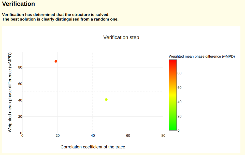
Verification is based on the idea that whereas there are many ways a solution may be incorrect, the true solution must be unique. In practice, we introduce realistic perturbations into the most probable solutions produced, then discrimination among the perturbed solutions and the ones presenting best figures of merit allows us to estimate the correctness of the solution produced. If incompatible solutions are not differentiated by their figures of merit, the solution will remain inconclusive. In ARCIMBOLDO_LITE perturbations generated include a random translation and reversed helices, while in ARCIMBOLDO_SHREDDER only a random translation is performed as we have not seen the case where tracing was reverting parts of the model.

Aims of the tutorial

This tutorial shows how to launch the coiled_coil mode^1,2 and predicted_model mode³ implemented in ARCIMBOLDO_SHREDDER⁴ in order to solve a 78 amino acids structure at 3.3 Å using a prediction obtained with AlphaFold 2⁵ and analyse the output of the program. This example uses the ARCIMBOLDO_SHREDDER version released on July 2024 through CCP4⁶ and our website. This run was performed in a workstation with 8 cores and took less than 3 hours to complete. This structure can also be solved with ARCIMBOLDO_LITE⁷ in its coiled_coil mode: see tutorial here.

Data tutorial

Experimental details

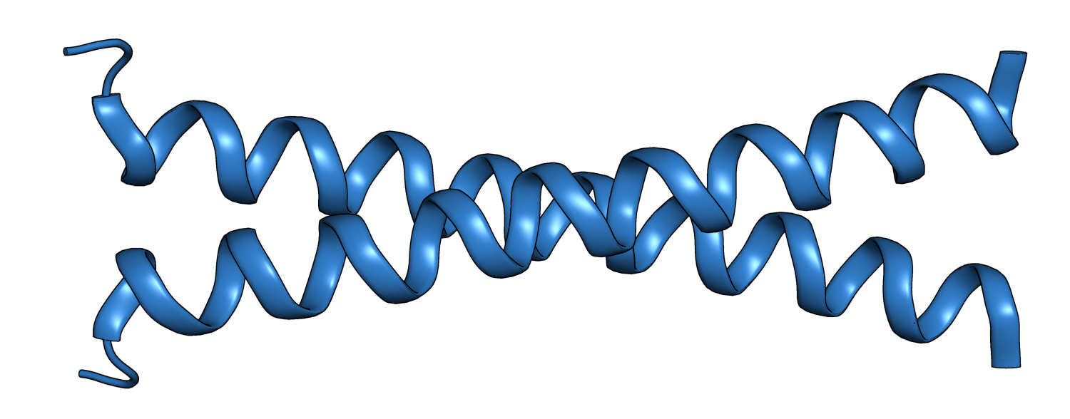
Test data for our tutorial is the crystal structure of the VBP Leucine Zipper with bound arylstibonic acid. This is a human transcription factor in complex with an inhibitor. The structure, composed by 2 ɑ-helices wrapped around each other to form a coiled coil domain, is deposited in the Protein Data Bank⁸ under the PDB code 4U5T9.

Crystallographic details are summarized in the following table:

Figure 1. Cartoon representation of PDB entry 4U5T. This figure was prepared using PyMOL¹⁰.

Step by Step tutorial

For this tutorial we will need the reflection file in two formats (.mtz and .hkl) and the prediction that will be used as a model for the molecular replacement search (ranked_0.pdb). All required files can be downloaded here. After downloading ARCIMBOLDO_SHREDDER Spheres (see instructions here), you are ready to follow this tutorial.

Required input

We need 4 files in order to run ARCIMBOLDO_SHREDDER Spheres:

Configuration .bor file:

The configuration file looks like follows:

[CONNECTION]:
distribute_computing: multiprocessing
setup_file: /path/to/setup.bor

[GENERAL]:
working_directory: /path/to/working_directory
mtz_path: %(working_directory)s/4u5t.mtz
hkl_path: %(working_directory)s/4u5t.hkl

[ARCIMBOLDO]
name_job: 4u5t
molecular_weight: 9340
number_of_component: 1
f_label: FOBS
sigf_label: SIGFOBS
number_of_component: 1
model_file: /absolute/path/to/ranked_0.pdb
coiled_coil: true
predicted_model: true

[LOCAL] 	
path_local_phaser: /path/to/phaser
path_local_shelxe: /path/to/shelxe

The [CONNECTION] section specifies the computing system used and the file containing the general configuration. The job can be run on a single machine (in multiprocessing) or in a local or remote grid of computers. If you want to run the job in multiprocessing you just have to change in the .bor file that you downloaded, the paths of the working directory, Phaser¹¹ and SHELXE¹² (in multiprocessing the setup_file is not required).

The [GENERAL] section contains the .mtz and .hkl file paths as well as the working directory where results will be written.

In the [ARCIMBOLDO] section all parameterization for the job is specified:

The name of the job that will be also the name of the output .html file.

The molecular weight and number of components should be defined for the Phaser search. In this case we set one number of components as we are considering both chains in the molecular weight specified. The default starting rmsd for predicted models is 0.8 Å (rmsd_shredder), but you can modify this value. The starting rmsd plays a prominent role in shredder, as it is used both for selecting the size of the models since it conditions the eLLG¹³ and Phaser’s target functions in the searches. Moreover, in successive cycles of gyre¹⁴ and gimble¹⁴ refinement the rmsd is decreased by 0.2. Thus, the rmsd used in translation search and rigid body refinement will typically be the set rmsd -0.2 Å.

It is also required to provide label identification in the .mtz file provided for either the amplitudes (F) and their sigmas (SIGF) or the intensities (I) and their sigmas (SIGI) used. If available, intensities are preferred. An .mtz file is a binary file but programs like MTZDMP¹⁵ available from the CCP4 suite can display their content.

If we are looking for more than one copy in the asymmetric unit we need to define it with the keyword fragment_to_search. In this case, we will look for only one copy as our search model already contains both chains.

The definition of the size of the models (sphere_definition), and the settings of model refinement strategies such as gyre and gimble. In this case, we will use default values.

The shelxe_line command line for the SHELXE steps in the algorithm can be defined. If unset, resolution-dependent default values and a specific parameterization for coiled coils will be used.

It is important to activate the predicted_model mode that entails:

Starting RMSD set to 0.8 Å (rmsd_shredder: 0.8). Notice that this value corresponds to an rmsd of 0.6 Å for the translation search and rigid body refinement.

Expected log likelihood gain (eLLG_target: 60).

Model preparation: B-factor standardization, keeping side chains, removal of unstructured areas, filtering of partial models to include domains.

Model-free verification: systematic elimination of the search model rendering traces exclusively outside the area occupied by the model to avoid model bias. When the coiled_coil mode is activated, a specific verification for those structures is performed.

It is important to activate the coiled_coil mode that entails:

VRMS calculation in the refinement step to optimize the RMSD parameter in order to maximize the LLG.

Disable placing pairs of tNCS related helices, as the internal periodicity of a single helix makes it difficult to differentiate genuine intermolecular tNCS from Patterson artifacts. If no solution is achieved, the alternative should be tried.

Activation of Phaser’s packing filter at translation, so at least one translated solution will pass the packing check.

SHELXE with helical sliding, which improves the autotracing of the coiled coil structures.

Final verification step, an additional step that generates perturbations (random translation) of the substructure leading to the best solution and compares their scores before and after extension. At resolution below 2 Å it was frequently observed that wrong placements of the helical fragments are not distinguishable from the Phaser figures of merit. This will be only activated at resolution worse than 2Å.

Finally, in the [LOCAL] section, the paths to Phaser and SHELXE are set. This is only required if you are in multiprocessing mode (run on a single computer), otherwise the paths must be specified in the configuration setup.bor file.

Execution

You can run the program interactively, having the output displayed on the screen or do it in background, redirecting an input file and passing the output to a .log file.

1. Interactively:

ARCIMBOLDO_SHREDDER 4u5t.bor

2. In background:

nohup ARCIMBOLDO_SHREDDER 4u5t.bor >& logfile.log;

Output and Results

In the directory where you launched ARCIMBOLDO_SHREDDER, you will find a directory called models containing a library of pdbs. Around each Calpha in the template, models are cut in a spatial way, producing a set of non-redundant, overlapping, compact models. In the default mode, they are also annotated in different chains in order to decompose them and perform gyre and gimble refinement, aiming to give more degrees of freedom and obtain a more accurate model. Also you will find an html output with a link to the html output of the library search. The first section echoes all parameters used for the run, so that defaults are listed along with values for the parameters set through the .bor file. This allows to reproduce the run even if defaults may change in future versions.

The directory called ARCIMBOLDO_BORGES contains the output of the ARCIMBOLDO_BORGES¹⁶ run using the library in models. The html output of the library search is found here. The next section displays a graph and a table summarizing the rotation clustering step as in ARCIMBOLDO_BORGES. A sortable table follows, summarizing the results for all Phaser and SHELXE steps, including top and average figures of merit for each rotation cluster that has been evaluated.

Figure 2. Interactive table with the figures of merit from Phaser and SHELXE for each rotation cluster.

After the table, you can find the backtrace and figures of merit for the best solution, in this case the structure is solved with a CC of 51.56% and 72 residues traced. Also, there are links to access the best scoring solution: the .pdb of the traced structure and its map in .phs format.

Figure 3. Backtracking of the model that leads to a correct solution.

After backtracking, a verification graph indicates that the structure is solved. It is crucial to check this verification result to ensure the reliability of the generated structural hypothesis. In this case, the best solution is clearly distinguishable from a random one.

Figure 4. Verification step graph.

Finally, the last section of this html containing a full configuration file will be reported, showing the parameterization used to launch the library of fragments. It includes all parameters, the ones provided by the user as well as the defaults that remained unchanged, and the log file of the run.

References

1. ARCIMBOLDO on coiled coils. Caballero, I., Sammito, M., Millan, C., Lebedev, A., Soler, N. and Uson, I.
   

   Acta Cryst. D74, 194-204 (2018) (doi:10.1107/S2059798317017582)

2. ARCIMBOLDO at low-resolution: Verification for coiled-coils and globular proteins. Caballero I., Castellví A., Triviño J., Jiménez E., Soler N., Borges R. and Usón I.
   

   Protein Sci. 33(9), e5136 (2024) (doi:10.1002/pro.5136)

3. Verification: model-free phasing with enhanced predicted models in ARCIMBOLDO_SHREDDER. Medina, A., Jiménez, E., Caballero, I., Castellví, A., Triviño Valls, J., Alcorlo, M., Molina, R., Hermoso, J. A., Sammito, M. D., Borges, R. & Usón, I.

   Acta Cryst. D78, 1283–1293 (2022) (doi:10.1107/S2059798322009706)

4. Exploiting distant homologues for phasing through the generation of compact fragments, local fold refinement and partial solution combination. Millán, C., Sammito, M. D., McCoy, A. J., Nascimento, A. F., Petrillo, G., Oeffner, R. D., Domínguez-Gil, T., Hermoso, J. A., Read, R. J. and Usón, I.

   Acta Cryst. D74, 290-304 (2018) (doi:10.1107/S2059798318001365)

5. Highly accurate protein structure prediction with AlphaFold. Jumper, J., Evans, R., Pritzel, et al.

   Nature 596, 583–589 (2021) (doi:10.1038/s41586-021-03819-2)

6. The CCP4 suite: integrative software for macromolecular crystallography. Aguirre, J. et al.

   Acta Cryst. D79, 449-461 (2023) (doi:10.1107/S2059798323003595)

7. ARCIMBOLDO_LITE: single-workstation implementation and use. Sammito, M., Millán, C., Frieske, D., Rodríguez-Freire, E., Borges, R. J. and Usón, I.
   

   Acta Cryst. D71, 1921-30 (2015) (doi:10.1107/S1399004715010846)

8. RCSB Protein Data Bank: biological macromolecular structures enabling research and education in fundamental biology, biomedicine, biotechnology and energy. Burley, S. et al.
   

   Nucleic Acids Research, 47(D1), D464–D474 (2018) (doi:10.1093/nar/gky1004)

9. P6981, An Arylstibonic Acid, Is a Novel Low Nanomolar Inhibitor of cAMP Response Element-Binding Protein Binding to DNA. Zhao, J., Stagno, J.R., Varticovski, L., Nimako, E., Rishi, V., McKinnon, K., Akee, R., Shoemaker, R.H., Ji, X., Vinson, C.
   

   Molecular Pharmacology, 82 (5) 814-823 (2012) (doi:10.1124/mol.112.080820)

10. The PyMOL Molecular Graphics System.
    

    Version 1.5.0.4 Schrödinger, LLC. (https://pymol.org)

11. Phaser crystallographic software. McCoy, A. J., Grosse-Kunstleve, R. W., Adams, P. D., Winn, M. D., Storoni, L. C. and Read, R. J.
    

    J. Appl. Crystallogr. D40, 658-674 (2007) (doi:10.1107/S0021889807021206)

12. Modes and model building in SHELXE. Usón, I. & Sheldrick, G. M.
    

    Acta Cryst. D80 (Pt 1), 4–15 (2024) (doi:10.1107/S2059798323010082)

13. On the application of the expected log-likelihood gain to decision making in molecular replacement. Oeffner, R D, Afonine, P. V, Millán, C., Sammito, M., Usón, I., Read, R. J., & McCoy, A.
    

    J. Acta Cryst. D74 (Pt 4), 245–255 (2018) (doi:10.1107/S2059798318004357)

14. Gyre and gimble: a maximum-likelihood replacement for Patterson correlation refinement. McCoy, A. J., Oeffner, R. D., Millan, C., Sammito, M., Uson, I. and Read, R. J.
    

    Acta Cryst. D74, 279-289 (doi:10.1107/S2059798318001353)

15. Overview of the CCP4 suite and current developments. Winn, M.D. et al.
    

    Acta Cryst. D67, 235-242 (2011) (doi: 10.1107/S0907444910045749)

16. Exploiting distant homologues for phasing through the generation of compact fragments, local fold refinement and partial solution combination. Millán, C. , Sammito, M. D., McCoy, A. J., Nascimento, A. F., Petrillo, G., Oeffner, R. D., Domínguez-Gil, T. , Hermoso, J. A., Read, R. J. and Usón, I.
    

    Acta Cryst. D74: 290-304 (2018) (doi:10.1107/S2059798318001365)